Pattern-Based FPC Routing Algorithm for Optimized Flexible PCB Design(Part I)

Flexible printed circuits (FPCs) are a specialized type of printed circuit board increasingly used in miniaturized and diversified electronic products. As applications expand, FPC designs have become more complex. Unlike conventional PCB routing, FPC routing faces stricter constraints and highly irregular routing spaces.
FPC Routing Challenges
In FPC layouts, components are densely concentrated within fan-out regions, resulting in uneven routing resource distribution. Component placement is often scattered and irregular, while interconnections between fan-out regions are complex.
Limitations of Existing Routing Methods
Direct application of conventional automatic routing algorithms leads to poor resource utilization, congestion at routing bottlenecks, and increased routing time. Therefore, routing planning is a critical stage in automated FPC design.
Traditional PCB routing planning primarily focuses on initial layer allocation.
Prior studies have addressed this problem using optimization methods such as transforming bus escape routing into maximum matching problems with polynomial time complexity, constructing routing maps through dynamic grids, or resolving bus conflicts via hierarchical algorithms.
Some approaches analyze routing from device topology or consider both internal and external bus conflicts.
However, these methods mainly target PCB motherboards containing large chips (e.g., BGA packages) and often neglect smaller components.
In contrast, FPCs mainly serve interconnection functions and consist largely of small- to medium-sized devices.
As a result, PCB routing strategies cannot be directly applied to FPC scenarios.
Existing FPC routing methods partition the routing space into regions based on pin locations, model connectivity using undirected graphs, and apply Dijkstra-based topology planning combined with heuristic boundary crossing optimization.
However, these approaches evaluate fan-out routability using simplified topological connections and overlook the practical impact of devices and existing routes on available routing resources.
Proposed Pattern-Based Routing Algorithm
To address these limitations, this paper proposes a pattern-based FPC routing planning algorithm.
Pattern routing is used to rapidly simulate real routing resource allocation within fan-out regions, preventing local resource shortages.
Routing patterns derived from manual design experience determine routing order, while Dijkstra's algorithm establishes non-intersecting topological sequences between fan-out regions to optimize channel resource allocation.
A hierarchical cost function dynamically determines layer assignment based on routing outcomes and network interactions.
By comparing global routing evaluation metrics across multiple routing modes, the optimal planning result is selected to guide detailed routing.
Experimental results demonstrate that the proposed method improves both routing efficiency and final routing quality.
Problem Description
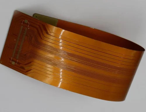
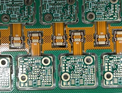
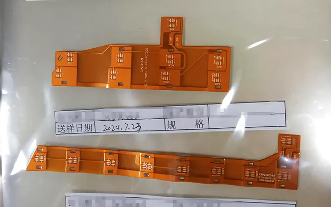
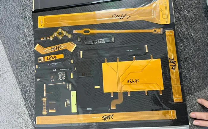
An actual industrial FPC board is shown in Figure 1.

Fig.1 Partition of an actual industrial FPC
To facilitate planning, the board is divided by partition lines into several fan-out areas (PinArea, PA) and channel areas (Channel).
FPCs often have multiple routing layers; a simplified 3D diagram of a channel area is shown in Figure 2.

Fig.2 Simplified stereograph view of the channel
A cross point (CP) is a point on the dividing line that connects the routing results of the pin area to those of the channel area.
Therefore, the routing results for the entire board can be decomposed into pin area routing and channel area routing, so that the automated routing process becomes start point–cross point 1–cross point 2–end point.
In this process, the segments connecting the start point and the end point to the cross points, respectively, constitute fan-out region routing and are subject to fan-out region routing constraints;
the segments connecting the cross points constitute channel region routing and are subject to channel region routing constraints.
The selection of cross point locations directly affects the overall detailed routing results; therefore, it is necessary to optimize the selection of cross point locations.
In summary, the FPC routing planning problem can be described as follows:
Inputs: FPC edge chain information O, pin coordinate information P, device information D, partition line L, and a set of two-terminal line networks N: ∈ N, where ni represents a two-terminal line network.
Constraints: Minimum spacing constraint between line networks; no vias allowed in channel zones.
Output: Information on the floor level and specific coordinates of the lines, grids, and points.
Algorithm Flowchart
Figure 3 illustrates the algorithm workflow proposed in this paper.

Fig.3 The overall flow of our method
First, the various necessary input data are preprocessed to obtain the routing mode, routing order, and routing direction for each fan-out zone.
Next, under the current fan-out mode, individual line networks are routed sequentially according to the current routing mode.
During routing, layer allocation is performed based on a comprehensive evaluation of the routing parameters of each wire mesh on every layer and its impact on other wire meshes;
after one iteration of the routing mode is completed, the crossing point positions on the corresponding partition lines are optimized for wire length.
By iterating through all design modes, we obtain the routing results and crossing positions that minimize the cost.
Finally, since the large mesh granularity may cause routing failures for a small number of line networks, it is necessary to perform post-processing on the failed routing networks.
The final failed routing networks are inserted into the set of crossing points on the partitioning lines according to the routing order of the current optimal mode, while ensuring that the topological order of non-intersection is maintained.
This ultimately yields the corresponding crossing point coordinates and crossing point correspondence relationships on the partitioning lines.
Routing Patterns
Patterned routing, also referred to as regular-pattern routing, originates from integrated circuit (IC) routing research.
The method is termed pattern routing because routing paths form regular geometric structures within the network.
Common routing patterns include L-shaped and zigzag configurations, which are generally categorized as monotonic and non-monotonic patterns.
Monotonic routing effectively reduces wire length, improving resource efficiency and space utilization.
In FPC fan-out regions, routing is constrained by numerous obstacles, limited routing layers, and unevenly distributed resources.
Therefore, routing algorithms must incorporate strong obstacle-avoidance capabilities to maximize resource utilization.
However, applying simple L-shaped or Z-shaped routing to single-net routing can sometimes waste routing resources and negatively impact subsequent routing tasks.
To address this issue, the single-wire tree routing method proposed in this work is built upon the A* routing framework.
The search space is restricted to four directions, enabling multi–Z-shaped routing while maintaining computational efficiency.
To enforce monotonic routing, searches in directions opposite to the target endpoint are prohibited.
Additionally, a turning cost is introduced to penalize excessive zigzagging, thereby favoring routing solutions with fewer bends.
Routing modes represent high-level strategies for constrained routing. Previous studies have proposed multiple routing modes that limit parameters such as routing direction and wire looping.
By constraining the search space, these modes significantly reduce the grid search complexity of traditional automatic routing algorithms, improving routing efficiency while still producing reasonable and potentially optimal solutions.
› Routing Patterns for Two Fan-Out Regions
In actual routing, the network consists of two fan-out regions, and the same operations must be performed on both regions.
If the routing order and node-passing sequence of only one fan-out region are used to determine the overall routing result, this may lead to poor routing results for the other fan-out region.
Therefore, a better approach is to conduct a comprehensive evaluation by simultaneously considering the routing patterns of both fan-out regions.
Given K wiring networks , where the starting and ending pins of these K networks are respectively located in fan-out region PA1 and fan-out region PA2, assume that in the example, the left fan-out area is PA1, with the fan-out direction to the right, and the right fan-out area is PA2, with the fan-out direction to the left; other directions can similarly be converted based on clock relationships.
PA1 and PA2 belong to different coordinate systems;
the lower-left corner of each is the origin (0,0), and the upper-right corners are (M1-1, N1-1 )and (M2-1, N2-1), respectively. Figure 4 shows an example of a single-layer grid layout for two fan-out regions connected by 8 lines.
In this figure, white grid points represent grid points that can be traversed by pattern routing; black grid points represent the starting points of pins on this layer;
blue grid points represent nodes occupied by obstacles and cannot be selected;
red straight lines are partition lines; and red grid points are candidate crossing points.
As shown in Figure 5, four routing modes were designed in this paper.

Fig.4 Example of two pin areas connected by 8 nets

Fig.5 Routing patterns of the interconnected pin areas
① Left-Down Mode (see Figure 5(a)).
In this mode, the left fan-out area serves as the reference fan-out area.
The pin routing order of the left fan-out area is used as the routing order for the right fan-out area.
Pins are scanned vertically from bottom to top in the left fan-out area, while horizontally, each row is scanned from left to right, the routing order shown in Figure 4 is .
② Left Up mode (see Figure 5(b)).
In this mode, the pin routing order of the left fan-out zone is used as the routing order for the right fan-out zone.
The vertical direction of the left fan-out zone is scanned from top to bottom, while the horizontal direction is scanned from left to right for each row.
Therefore, the routing order shown in Figure 4 is .
③ Right Down mode (see Figure 5(c)).
This mode uses the pin routing order of the right fan-out zone as the routing order for the left fan-out zone.
It scans vertically from bottom to top in the right fan-out zone while scanning horizontally from right to left for each row. Thus, the routing order for the example in Figure 4 is .
④ Right Up mode (see Figure 5(d)).
In this mode, the pin routing order of the right fan-out region is used as the routing order for the left fan-out region.
The scan proceeds vertically from top to bottom in the right fan-out region, while horizontally scanning each row from right to left.
Thus, the routing order shown in Figure 4 is .
Multi-Mode Routing Strategy
Since four routing sequence modes are designed for the routing phase, it is necessary to route the entire network four times and select the instance with the lowest cost. Let denote the line networks to be routed, where 1 ≤ ni ≤ nk ≤ K.
For any two of these networks, in both the Left-Down and Right-Down modes, the right fan-out region and the left fan-out region follow the same principle: starting from the lowest candidate crossing point, and the networks are routed in sequence according to the routing order, selecting the candidate crossing point with the smallest y-coordinate as the endpoint.
This ensures that the y-coordinate of the candidate crossing point for nj is always above that of ni. If the pins of both fan-out networks are successfully routed, the routing is successful; otherwise, it fails.
The Left Up mode works similarly to the Right Up mode: the wire mesh selects the candidate crossing point with the largest y-coordinate as the endpoint in the routing order to perform mode routing.
Routing Results and Mode Selection
Figure 5 shows the routing results for the four routing modes in the example in Figure 4.
In the Left Down mode, all lines are routed successfully, while in the Left Up mode, only 5 line networks are routed; in the Right Down mode, 6 line networks are routed; and in the Right Up mode, 7 line networks are routed.
In summary, the Left Down mode should be selected for the routing result.